CT Analysis API: Making Pylinac Honest About Catphan QA

The Problem With Trusting a Single Slice

CT acceptance testing and periodic QA both come down to the same ritual: scan a Catphan phantom, run it through analysis software, and get back HU accuracy, uniformity, spatial resolution, and low-contrast detectability. Pylinac is the open-source tool most medical physicists reach for to do that. It’s well tested and widely trusted — and it also makes a handful of assumptions that don’t survive contact with a shelf of scanners from different vendors, loaded by different technologists, on different days.

It assumes the phantom always goes into the bore the same way round. It samples HU on a single slice, so a borderline material can flip from pass to fail depending on which slice the anchor search happened to land on. And its slanted-wire MTF picks the brightest pixel in the image, which works until a CTP404 wire ramp or a streak off a dense plug is brighter than the actual wire.

None of these are edge cases you’d catch by eye on one scan. They’re the kind of thing that shows up as noise in a longitudinal trend, or as a script that works on the reference scan and silently misbehaves on the next one.

The CT Analysis module in the X-ray Imaging Analysis Toolkit wraps Pylinac’s Catphan implementation, fixes each of these, and — because none of it is useful if it only runs inside a browser tab — exposes the entire pipeline as a plain Python function you can call from a batch job.

The Analysis Pipeline

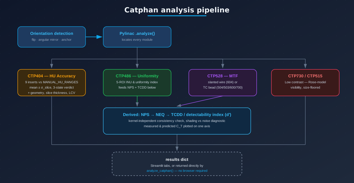
Every Catphan family member (604, 504, 503, 600, 700) runs the same sequence: orientation detection first, then Pylinac’s own module localisation, then four families of measurement that feed two derived layers.

CT analysis pipeline: orientation detection, Pylinac module localisation, HU/uniformity/MTF/low-contrast measurement, and the NPS/TCDD/NEQ/detectability derived layer

Phantom	CTP404 HU	CTP486 Uniformity	CTP528 MTF	Low Contrast
Catphan 604	9 inserts, corrected angles	✅	Slanted wire (5°, 50 μm)	CTP730 — 3 contrast levels
Catphan 504 / 503 / 600 / 700	9 inserts	✅	TC bead (0.18 mm)	CTP515

Orientation Detection and the Angular Mirror

Pylinac assumes a fixed mapping between slice order and physical module position. Load the phantom head-to-foot instead of foot-to-head and every declared module offset has the wrong sign — localisation fails silently rather than loudly.

The fix runs in four steps. First, every slice gets a per-slice σ_HU profile inside the central 0.85 R circle, dropping slices where the phantom fills less than 95% of that circle (the true guard — a mean-HU test can’t catch end-cap-plus-air slices that read a plausible −93 HU but carry an implausibly high σ). Second, the CTP404 plateau is found: the contiguous high-σ region whose slices also carry the sensitometry signature — a minimum below −800 HU (genuinely air) and a maximum more than 400 HU above the median (a dense insert). Third, whichever side of that plateau holds more phantom slices tells you where the rest of the phantom lies, compared against the side the declared offsets point to — read from each phantom class’s own modules dict, because Pylinac isn’t self-consistent about the sign (CTP486 sits at −110 mm on the 503, −65 on the 504, but +80 on the 604).

Fixing slice order isn’t the whole problem, though — a phantom rotated 180° about the vertical axis also mirrors the image, θ → 180 − θ, which maps every HU insert onto the wrong plug. OrientationMixin._resolve_mirror() decides this per scan, independent of the flip:

A manual sidebar override always wins.
Otherwise, place the HU-module ROIs both ways round on the CTP404 slice and keep whichever layout gives the lower mean |measured − nominal| across all nine inserts. On the reference 604 scan that’s 20 HU for the correct layout against 491 HU for the wrong one — not a delicate call.
Fall back to the DICOM PatientPosition tag when the scoring is inconclusive.

Multi-Slice HU Sensitometry

Pylinac measures CTP404 HU accuracy on a single slice. Each insert carries a few HU of slice-to-slice noise, which is enough on its own to move a borderline material across its acceptance boundary depending on nothing but which slice the anchor search landed on — and that’s not any one material’s quirk, it’s a property of single-slice sampling that all nine inserts are exposed to. On the reference 604, two different materials show it in opposite directions: Teflon reads 938.5 HU on one slice — a fail against its 941 HU lower bound — and 941.6 ± 3.2 HU averaged over five slices, a pass. Air does the same trick the other way round: −986.0 HU on one slice sits exactly on its bound, while −984.0 ± 1.3 HU averaged is a fail (that particular excursion turns out to be the scanner’s own air-calibration baseline, not a measurement error — the rod core still reads −988.6 HU with a tight ROI).

Each insert is instead sampled over anchor ± 2 mm, converted to slices at run time, and scored against MANUAL_HU_RANGES — asymmetric per-material ranges transcribed from the manufacturer manual, replacing Pylinac’s symmetric ±HU defaults:

Material	Nominal HU	Published Range
Air	−1000	−1046 to −986
PMP	−196	−220 to −172
LDPE	−104	−121 to −87
Poly	−47	−65 to −29
Acrylic	115	92 to 137
Delrin	365	344 to 387
Teflon	1000	941 to 1060
20% Bone	237	211 to 263
50% Bone	725	667 to 783

The verdict is three-state rather than a boolean pass/fail:

Verdict	Meaning
✅ pass	Mean sits inside the band
⚠️ warning	Outside, but `mean ± σ_slice` still reaches into it — marginal, not demonstrably out
❌ fail	Outside even allowing for that spread

Note these published ranges aren’t a tolerance — the manufacturer’s own footnote states they’re the spread from 94 scans across different scanners at 120 kVp, and “numbers outside of this range are not unusual.” The tool reports the excursion; deciding whether it’s actionable stays the physicist’s call, made against their own baseline. That disclosure travels with every result, in the panel caption, the badge’s help text, and the CSV export.

Robust Slanted-Wire MTF

The Catphan 604 measures spatial resolution with a 50 μm tungsten wire tilted 5° off the scanner’s z-axis. Pylinac’s stock localiser picks the brightest pixel in the phantom, excluding only the HU-plug annulus — which sounds reasonable until a clinical scan shows the wire peaking around 550 HU at the same time as the CTP404 wire ramps and streaks off the Teflon and bone plugs. Which one wins depends on the anchor slice, and MTF₅₀ moved by 2× across a ±6-slice range in testing.

CTP528CP604Robust replaces both halves of the pipeline. Localisation runs by persistence: the true wire drifts by tan(5°) × slice spacing per slice — under a pixel across the whole stack — so it lands at the same (x, y) in every slice, while the ramps sweep roughly 2°/slice and the streak maxima hop around at random. A consensus vote across slices finds the wire; if nothing recurs in at least 60% of slices, the class raises rather than returning a number. The PSF construction changes too: instead of one patch per slice radially averaged into 1-pixel bins (only five samples for a 3 mm patch at 0.78 mm pixels), every pixel of every slice is pooled as an individual (radius, value) sample about that slice’s own sub-pixel wire centre, binned at 0.25 px (OversampledWireMTF).

The anchor-sensitivity test is the one that matters: across six different anchor slices on the reference 604, Pylinac’s brightest-pixel finder gives MTF₅₀ anywhere from 0.199 to 0.392 lp/mm, with MTF₁₀ undefined in two of the six runs. CTP528CP604Robust gives 0.391–0.414 lp/mm, MTF₁₀ defined every time.

Low-Contrast Rods: Contrast Isn’t Detectability

The low-contrast modules (CTP730 on the 604, CTP515 elsewhere) score whether a rod is visible, and visibility is not the same thing as contrast. The Rose-model visibility used for the actual verdict is:

$V = \frac{\Delta\text{HU} \cdot \sqrt{N}}{\sigma_{\text{bg}}}$

with N the pixel count in the rod’s ROI. The $\sqrt{N}$ term is the whole point — a large rod integrates more independent samples, so it’s detectable at a contrast a small rod isn’t, and a plain contrast-to-noise ratio can’t express that. Contrast itself is reported as a signed HU difference rather than Pylinac’s default Michelson ratio, which is meaningless for CT numbers (they sit near zero and can be negative — a singular denominator waiting to happen):

$C = |\text{HU}_{\text{rod}} - \text{HU}_{\text{bg}}|, \qquad \text{CNR} = \frac{|\text{HU}_{\text{rod}} - \text{HU}_{\text{bg}}|}{\sigma_{\text{bg}}}$

Two scoring rules keep the headline number honest. Rods whose ROI holds fewer than 16 pixels (below the manufacturer’s own “at least 4×4 pixels” floor) are excluded rather than scored — at the reference 604’s 0.781 mm pixels, the 2 mm rod ROI holds four pixels total, where $\sqrt{N}$ in the visibility formula is noise dressed as a number. And the reported figure isn’t the smallest rod that happens to score above threshold — visibility isn’t monotonic in practice, so a single small rod scoring high on noise would misreport the group. Instead it’s the smallest diameter at which every larger scoreable rod is also visible: on the reference 604’s 1.0% group, rods are visible at 15/9/8/7 mm, invisible at 6/5/4/3 mm, and visible again at 2 mm (where the ROI is four pixels) — the plain minimum would report 2 mm for a scan whose honest answer is 7 mm.

NPS, NEQ and the Detectability Index

The Uniformity tab runs a chain of derived metrics on the same CTP486 slice, each feeding the next: NPS → NEQ → TCDD.

The noise power spectrum is computed in-line from the DICOM arrays — up to 9 adjacent slices, 50% overlapping 64-px sub-ROIs per AAPM TG-233, big-ROI polynomial detrending — and reported un-normalised in HU²·mm² (no mean-signal normalisation, because HU is already an absolute, water-referenced scale):

$\text{NPS}_{2D}(u,v) = \frac{\Delta x\,\Delta y}{N_x N_y}\left|\text{DFT}[I_{\text{detrended}}](u,v)\right|^2$

Combining that with the CTP528 MTF gives the Noise Equivalent Quanta:

$\text{NEQ}(f) = \frac{\text{MTF}^2(f)}{\text{NPS}(f)}$

NEQ is kernel-independent by construction — a reconstruction kernel multiplies MTF by $|K|$ and NPS by $|K|^2$ , so NEQ cancels it exactly. That makes a sustained upturn a consistency check rather than a scanner property: it means the MTF has flattened onto its own noise floor rather than the scanner having genuinely improved at high frequency. The 503 triggers this at 0.461 lp/mm, where its bead MTF still reads 0.151 and never reaches the conventional 0.1 cutoff.

Threshold contrast detail detectability (TCDD) is measured statistically on the same slice, using $C_T(d) = 3.29 \times \sigma_\chi(d)$ (the 99.9% confidence level, not 95%), then fit to $C_T(d) = c/d^2 + b/d + a$ . Crucially, TCDD is measured on the acquired image while NPS is detrended — deliberately, because a radiologist can’t mentally subtract a shading gradient, so low-frequency shading is a genuine part of what limits detectability and belongs in the number. The detectability index $d'$ integrates MTF²/NPS against a disc task’s jinc-shaped spectrum for an ideal prewhitening observer, giving a predicted threshold contrast in closed form that’s plotted on the same axis as the measured TCDD curve. When the ratio between them widens with detail size, that’s the signature of shading-limited rather than noise-limited performance — on the reference scans, the 604 sits at 0.43–1.90× across 2–15 mm while the steeper-shaded 503 runs 0.86–3.86×.

A Streamlit-Free API

None of the above is useful if it only runs behind a file uploader. The package’s public entry point does the whole pipeline — orientation, Pylinac’s module analysis, and the NPS/TCDD/NEQ/detectability layer — without touching Streamlit at all:

from src.qa.ct_analysis import PHANTOM_CLASSES, analyze_catphan

results = analyze_catphan("scans/2026-08/cp604", PHANTOM_CLASSES["Catphan 604"])
print(results["hu"], results["integral_non_uniformity"])

analyze_catphan() accepts a directory of DICOM files, a ZIP path, or a list of file-like uploads, so a batch job, a longitudinal trending script, or the test suite can call it directly instead of reaching into private helpers or simulating a browser session. It takes the same anchor/flip/mirror overrides the sidebar exposes, and computes the derived metrics by default (derived=True) so a generated report isn’t silently missing NPS, TCDD, NEQ or d′ just because nobody scrolled to that tab. src/qa/ct_analysis/__init__.py imports Streamlit only inside the view function, so import src.qa.ct_analysis on its own costs nothing — the batch path and the interactive path share every line of analysis code and diverge only at the very last step, where one prints a dict and the other renders five tabs of it.

Under the Hood

Layer	Technology
Phantom analysis engine	Pylinac (pinned fork) — Catphan localisation, HU/MTF/uniformity/low-contrast primitives
Orientation & corrections	Custom `OrientationMixin` — flip detection, angular mirror resolution
Derived metrics	NumPy / SciPy — NPS, NEQ, TCDD, detectability index
Image processing	scikit-image, OpenCV
DICOM I/O	pydicom
Interactive UI	Streamlit
Batch / programmatic use	`analyze_catphan()` — Streamlit-free public entry point
Plotting	Matplotlib
Containerisation	Docker (multi-stage, conda builder for binary `pyarrow`)

Try It

The CT Analysis module is live inside the X-ray Imaging Analysis Toolkit — upload a Catphan DICOM series or ZIP, pick your phantom model, and let orientation detection sort out which way it was loaded.

A single slice can lie to you about whether a scanner passed. This one checks its own work before it tells you.