Flat Panel QA: A Complete Toolkit for Digital X-ray Detector Characterisation

Introduction

Characterising a flat panel X-ray detector properly means more than running a quick uniformity check. A thorough QA programme requires quantifying spatial resolution, frequency-dependent noise, dose efficiency, and contrast detectability — following the same international standard across every measurement so results are comparable and reproducible.

The X-ray Imaging Analysis Toolkit is a Streamlit web application that implements the complete flat panel QA pipeline defined in IEC 62220-1-1:2015. It operates on raw, unprocessed detector images (“FOR PROCESSING”) to measure intrinsic detector performance, independent of any manufacturer post-processing.

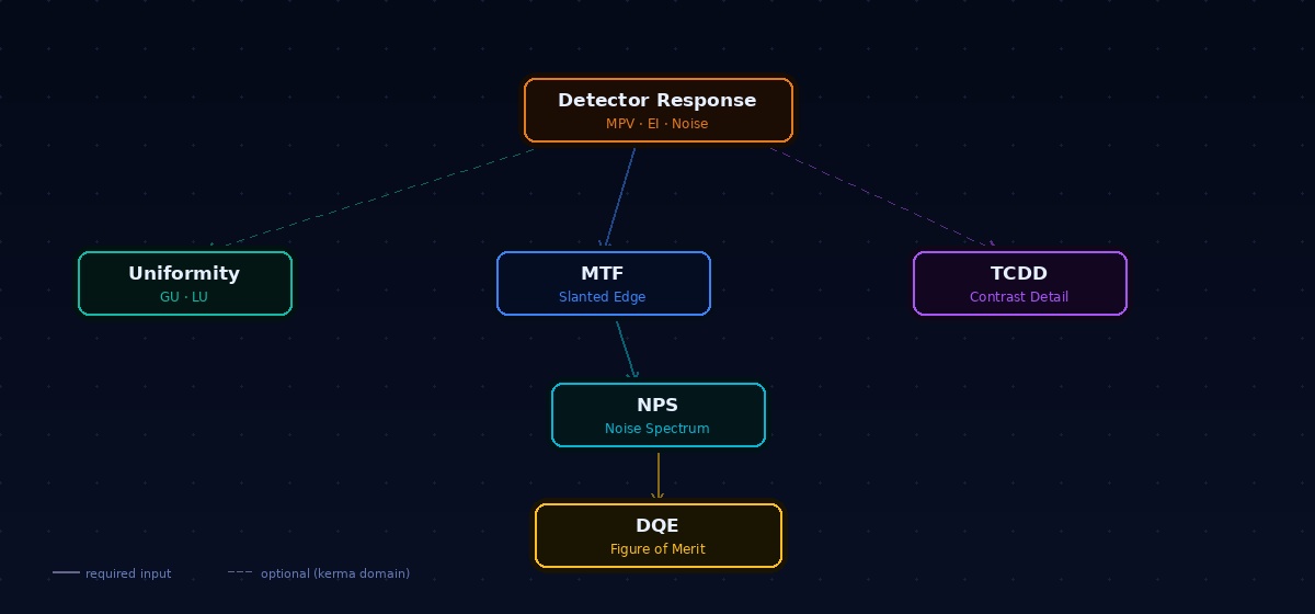
The Analysis Pipeline

The six modules form a logical dependency chain where earlier analyses feed directly into later ones. Solid arrows indicate required inputs; dashed arrows indicate the optional kerma-domain mode enabled when the detector response fit is available.

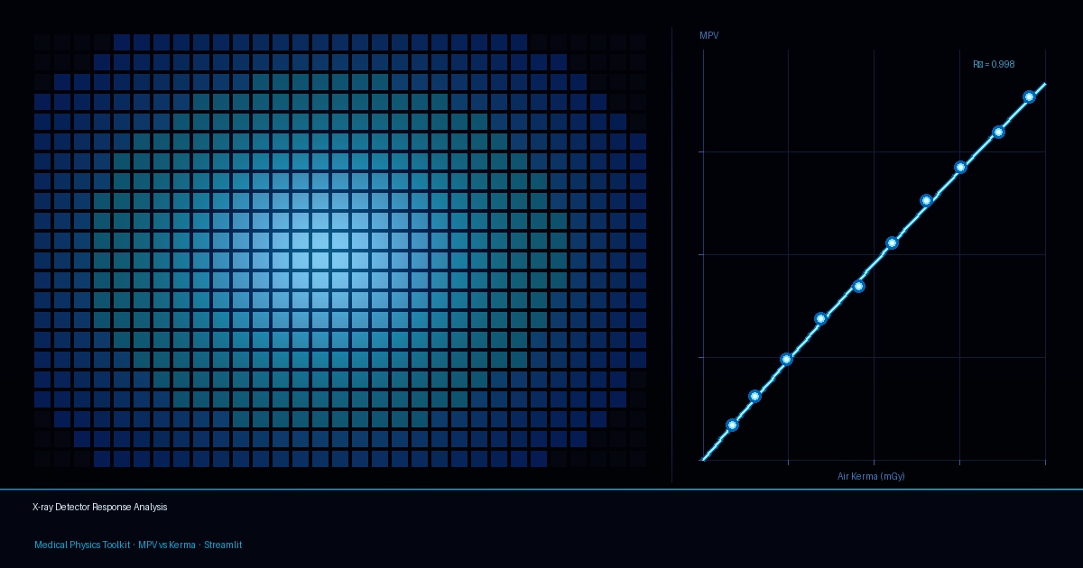
Analysis pipeline showing module dependencies

Detector Response Characterisation

Everything else depends on knowing how the detector converts incident radiation into digital output. This module takes a series of flat-field exposures acquired at different dose levels and fits the MPV vs Air Kerma relationship:

Image type	Fit model
RAW (linear encoding)	$\text{MPV} = a \cdot K + b$
STD (log-encoded)	$\text{MPV} = a \cdot \ln(K) + b$

The fit method can be auto-detected from the DICOM tag (0028,1040) PixelIntensityRelationship. Results are characterised by $R^2$ and maximum deviation. The fitted prediction function — and its inverse — are cached in session state for use by every downstream module.

The same set of exposures also yields two additional analyses:

EI vs Air Kerma — A linear fit of the IEC 62494-1 Exposition Index against kerma ( $\text{EI} = a \cdot K + b$ ), enabling cross-manufacturer exposure level comparisons.

Noise Decomposition — The total variance across the measured kerma range is decomposed into three physical components:

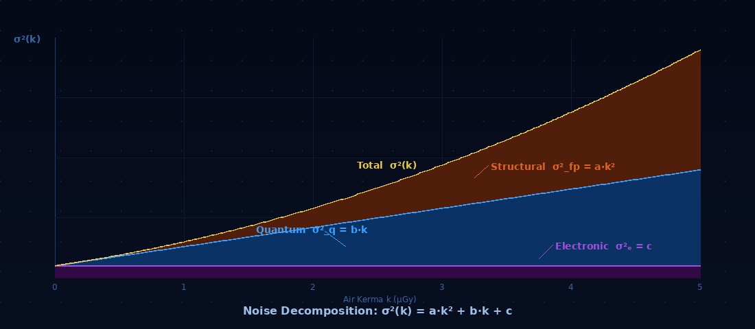
$\sigma^2(k) = \underbrace{a \cdot k^2}_{\substack{\text{Structural} \\ \text{(gain non-uniformity)}}} + \underbrace{b \cdot k}_{\substack{\text{Quantum} \\ \text{(Poisson-limited)}}} + \underbrace{c}_{\substack{\text{Electronic} \\ \text{(dark current, readout)}}}$

Noise variance components plotted against air kerma, showing structural (orange), quantum (blue), and electronic (purple) regions

The structural component is measured directly from $N \geq 2$ repeated exposures at a single reference kerma level $k_0$ using the division method (Monnin et al., Phys. Med. Biol. 59, 2014). Dividing each frame by the pixel-wise mean across all frames normalises out the multiplicative fixed-pattern noise, isolating the stochastic (quantum + electronic) component. Electronic and quantum components are then separated by weighted linear extrapolation of the stochastic variance to $k \to 0$ .

Spatial Uniformity

A 30 mm × 30 mm moving ROI slides across the central 80% of a flat-field image with a 15 mm step. For each position, MPV, SD, and SNR are computed. Two levels of uniformity are reported:

Global Uniformity (GU) — Maximum deviation of any ROI from the overall mean:

$\text{GU}_\text{PV} = \max_i \frac{\left|\text{PV}_i - \overline{\text{PV}}\right|}{\left|\overline{\text{PV}}\right|} \times 100\%$

$\text{GU}_\text{SNR} = \max_i \frac{\left|\text{SNR}_i - \overline{\text{SNR}}\right|}{\left|\overline{\text{SNR}}\right|} \times 100\%$

Local Uniformity (LU) — The same metric computed relative to each ROI’s 8 immediate neighbours. This catches localised defects that global metrics can miss.

When the detector response fit is available in session state, the analysis can run entirely in kerma domain, providing a physics-based uniformity assessment expressed in dose units rather than arbitrary pixel values.

Modulation Transfer Function (MTF)

Spatial resolution is measured via the slanted edge method specified in IEC 62220-1-1:2015. The user uploads one or two RAW images of a lead or tungsten edge phantom tilted slightly off-axis.

Algorithm:

Hough Transform detects the edge angle and orientation.
Pixel values are projected perpendicular to the edge to build the Edge Spread Function (ESF), oversampled by the slant angle.
The Line Spread Function (LSF) is computed as the numerical derivative of the ESF.
The MTF is the magnitude of the Fourier Transform of the LSF: $\text{MTF}(f) = \left|\mathcal{F}\{\text{LSF}\}\right|$ .

IEC 62220-1-1 requires edge angles of 3°–5° (horizontal) or 85°–87° (vertical). The UI reports angle compliance and flags any deviation from this range.

When two orthogonal edge images are provided, the module computes the geometric mean MTF:

$\text{MTF}_\text{geom}(f) = \sqrt{\text{MTF}_V(f) \times \text{MTF}_H(f)}$

This isotropic MTF is required as input to the DQE calculation.

Key metrics: $\text{MTF}_{50}$ (practical resolution limit) and $\text{MTF}_{10}$ (high-frequency cutoff), both in lp/mm.

Noise Power Spectrum (NPS)

The NPS quantifies frequency-dependent noise following IEC 62220-1-1:2015. One or more uniform flat-field images are accepted; multiple images improve statistical reliability (IEC recommends $\geq 4 \times 10^6$ total analysed pixels).

Algorithm:

A large central ROI (default 1024 px, adjustable 25–250 mm) is extracted from each image and subdivided into small ROIs (default 128 px).
Each small ROI undergoes a 2D FFT; power spectra are averaged across all ROIs and all images.
The result is normalised to yield the NNPS:

$\text{NNPS}(u,v) = \frac{\Delta x \cdot \Delta y}{N_x \cdot N_y} \cdot \frac{\left|\mathcal{F}\right|^2}{\mu^2} \quad [\mu\text{m}^2]$

Outputs: radial-average NNPS ( $\mu\text{m}^2$ ) for display, plus directional X and Y profiles for detecting anisotropic noise such as scan-line artefacts. The raw 1D NPS in mm² is cached for DQE computation. A warning is issued if the analysed pixel count falls below the IEC threshold.

Detective Quantum Efficiency (DQE)

DQE is the single figure of merit for a digital X-ray detector — it quantifies what fraction of the dose reaching the detector is actually converted into useful signal information. The IEC 62220-1-1:2015 working formula is:

$\text{DQE}(f) = \frac{\text{MTF}^2(f)}{\text{NNPS}(f) \cdot q \cdot K_a}$

where $q = 30174\ \text{mm}^{-2}\,\mu\text{Gy}^{-1}$ is the photon fluence per unit kerma for the RQA5 beam quality specified by the standard, and $K_a$ is the air kerma in $\mu\text{Gy}$ . NNPS here is the raw 1D NPS in mm².

Both MTF (geometric mean from two orthogonal edges) and NPS must be completed in the same session. The module interpolates them onto a common frequency grid (300 points across the intersection of their frequency ranges) and reports:

Metric	Meaning
$\text{DQE}(0)$	Low-frequency dose efficiency
$f$ at $\text{DQE} = 0.5$	Frequency at which half the input $\text{SNR}^2$ is preserved
$f$ at $\text{DQE} = 0.1$	High-frequency cutoff

Interpretation:

$\text{DQE}(0)$	Assessment
0.6–0.8	Excellent (modern CsI/a-Si or Se-based panels)
0.4–0.6	Good (well-maintained system)
0.2–0.4	Fair (ageing or suboptimal configuration)
< 0.2	Poor — investigation warranted

Threshold Contrast Detail Detectability (TCDD)

TCDD estimates the minimum detectable contrast as a function of detail size, using the statistical method described by Paruccini et al. (2021). It operates on a flat-field image independently of MTF and NPS, but like Uniformity it benefits from the detector response fit when available — optionally converting pixel values to kerma domain before computing contrast thresholds.

From a uniform flat-field image, sub-ROIs of varying size are sampled across the central $1024 \times 1024$ px region. For each detail size, the threshold contrast at 95% confidence is:

$C_T = 3.29 \times \sigma_\chi$

where $\sigma_\chi$ is the standard deviation of sub-ROI means at that size. Results are normalised to the mean signal and expressed as a percentage.

The contrast-detail relationship is fitted to $C_T(d) = c/d^2 + b/d + a$ , and key values at $d = 0.5\ \text{mm}$ and $d = 2.0\ \text{mm}$ are reported for cross-system comparison.

IEC 62220-1-1:2015 Compliance

IEC Requirement	Module	Implementation
Slanted edge MTF	MTF	Hough-based edge detection, ESF → LSF → FFT
Edge angle 3°–5° or 85°–87°	MTF	Angle detection with compliance flag
Geometric mean of orthogonal MTFs	MTF	Automatic when 2 images provided
NPS from $\geq 4 \times 10^6$ pixels	NPS	Multi-image support with pixel count warning
NNPS normalisation	NPS	$\text{NNPS} = \text{NPS}/\mu^2$ with unit conversion
$\text{DQE} = \text{MTF}^2 / (\text{NPS} \cdot q \cdot K_a)$	DQE	RQA5 $q = 30174\ \text{mm}^{-2}\,\mu\text{Gy}^{-1}$ , raw NPS in mm²
Detector response linearity	Detector Response	MPV vs kerma (linear or log), auto-detected from DICOM

Getting Started

All modules are available in the web application. Upload your DICOM or RAW flat-field and edge phantom images and run the modules in pipeline order — each result feeds the next.